Welcome to nlfem’s documentation!

Documentation

The implementation has a Python interface and a C++ core. The Python interface provides the main functionality. The C++ core documentation should provide sufficient insight to enable the user to extend nlfem, for example, by new kernel functions.

• Python interface docs

• C++ core docs

Build and Install

Docker

To quickly set up a terminal with an nlfem installation execute

docker run --interactive --tty registry.gitlab.uni-trier.de/pde-opt/nonlocal-models/nlfem:latest bash

The above image contains a Jupyter notebook installation. You can start a notebook which can be reached at http://localhost:<port> by

docker run -p <port>:80 registry.gitlab.uni-trier.de/pde-opt/nonlocal-models/nlfem:latest jupyter notebook

Manual Installation

Ubuntu 22.04 LTS

On Ubuntu the required packages can be installed by the following commands:

sudo apt-get update
sudo apt-get install git gcc g++ libarmadillo-dev liblapack-dev libmetis-dev python3-venv python3-dev libgmp-dev libcgal-dev
mkdir nlfemvenv
python3 -m venv nlfemvenv/
source nlfemvenv/bin/activate

The terminal will now indicate that you are in (nlfemvenv). In order to install nlfem run:

git clone https://gitlab.uni-trier.de/pde-opt/nonlocal-models/nlfem.git
cd nlfem
python3 -m pip install -r requirements.txt
python3 setup.py build install

Required packages

In general a system has to meet the following requirements.

1. The basic requirements are the programs gcc, g++, python3-dev, python3-venv, libgmp-dev, libcgal-dev, metis, libmetis-dev, libarmadillo-dev. You further need the Python 3 packages numpy and scipy. If you want to change the Cython code, you require the package Cython.

2. For running the examples you additionally need to install the Python packages matplotlib, meshzoo. Make sure to install the correct versions by using the requirements.txt.

License

nlfem is published under GNU General Public License version 3. Copyright (c) 2021 Manuel Klar, Christian Vollmann

---

Quick Start

To test the rates for the constant kernel run

cd nlfem/examples/test2D
python3 computeRates2D.py -s 4 -f testConfConstant

Run a test with other configurations by indicating the file e.g. -f testConfFull. The option -s indicates the number of refinement steps.

Usage

Let \(\Omega \subset \mathbb{R}^{d}, (d=1,2,3)\) be a bounded domain and \(\Gamma^D \subset \Omega^c\), where we allow that \(\Gamma^D = \emptyset\). The package nlfem allows to assemble stiffness matrices which discretize the nonlocal operator

\[-\mathcal{L}_\delta \mathbf{u}(\mathbf{x}) = 2\int_{\Omega \cup \Gamma^D} \mathbb{1}_{B_{\delta}(\mathbf{x})}(\mathbf{y}) \left(\mathbf{C}(\mathbf{x}, \mathbf{y})\mathbf{u}(\mathbf{x}) - \mathbf{C}(\mathbf{y}, \mathbf{x})\mathbf{u}(\mathbf{y}) \right)\]

where \(\mathbf{C} \in \mathbb{R}^{n\times n}, (n \geq 1)\) is a possibly matrix-valued integral kernel and \(B_{\delta}(\mathbf{x})\) a \(p\)-norm ball (\(p \in [1, \infty]\)) of radius \(\delta\). Details about the mathematical background of nlfem are presented in [Klar2022].

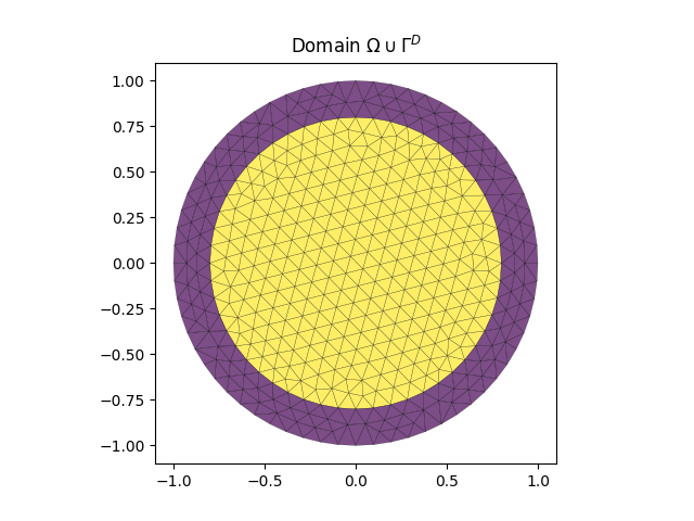
Example We exemplify the usage of nlfem by solving a scalar, nonlocal Dirichlet-type problem

\[\begin{split}\begin{cases} -\mathcal{L}_\delta u(\mathbf{x}) = f_{\Omega}(\mathbf{x}) & \mathbf{x} \in \Omega\\ u(\mathbf{x}) = g(\mathbf{x}) & \mathbf{x} \in \Gamma^D \end{cases}\end{split}\]

where \(\Omega\) by a 2d-disk of radius 0.9 with a nonlocal boundary \(\Gamma^D\) of width \(\delta=0.1\).

Finite element mesh

The construction requires a finite element mesh in a 1d, 2d, or 3d domain. The mesh is characterized by its elements and vertices. The elements are given by a numpy.ndarray of datatype np.int_ and shape (nE, d+1), where nE is the number of elements and d the dimension of the domain. The vertices are a numpy array of floats with shape (nV, d), where nV is the number of vertices.

The domain described by the the above arrays needs to be divided into different parts according to their purpose. To that end we define a numpy nd.array called elementLabels of type np.int_ and length nE. It assigns a label to each element. Negative elements indicate the Dirichlet boundary, any positive element is considered a part of the domain and zero labeled elements are not part of the integration.

Example The finite element mesh (that is vertices and elements) of the required form can be obtained for example from gmsh. In the example the elementLabels are set to -1 on \(\Gamma^D\) (blue in the below figure) and 1 on \(\Omega\) (yellow). The plot is based on a domain saved in examples/docs/mesh.pkl.

import pickle
import matplotlib.pyplot as plt

mesh_arrays = pickle.load(open("mesh.pkl", "rb"))
elements, vertices, elementLabels = mesh_arrays["elements"], mesh_arrays["vertices"], mesh_arrays["elementLabels"]

plt.tripcolor(vertices[:, 0], vertices[:, 1], elements, facecolors=elementLabels, edgecolors="black", linewidth=.2, alpha=.7)
plt.title(r"Domain $\Omega \cup \Gamma^D$")
plt.gca().set_aspect('equal')
plt.savefig("domain.png")
plt.close()

Settings

The kernel is a dictionary which contains the keys function, horizon, outputdim and possibly fractional_s. A list of implemented kernel functions can be found via show_options(). The horizon determines the interaction radius of the kernel and outputdim tells whether the kernel is scalar or matrix-valued. Given the kernel has a singularity which requires regularizing integral transformations we need to determine the parameter s of the singularity in fractional_s. The quantity is required for the special integration routines fractional and weakFractional which need to be applied to those kernels.

Example We choose a scalar kernel of truncated fractional type

\[C(\mathbf{x}, \mathbf{y}) = \frac{2-2s}{\pi\delta^{2-2s}} \frac{1}{|\mathbf{x}-\mathbf{y}|^{d + 2s}}\]

where \(d=2\) and \(s=0.4\). The corresponding dictionary reads as

kernel = {
    "function": "fractional",
    "horizon": 0.1,
    "outputdim": 1,
    "fractional_s": 0.4
}

As optional parameter it is possible to hand over varying kernel coefficients with the key "Theta". Of course, the implemented kernel has to support the usage of the given information. This is so, for example, for the kernel functions "theta" and "sparsetheta" which evaluate

\[\frac{4}{\pi \delta^{4}} \Theta(x,y)\]

and

\[\frac{4}{\pi \delta^{4}} (1 - \Theta(x,y)),\]

respectively. The coefficients Theta are expected to be of type scipy.sparse.csr_matrix. However, there are no other restrictions, so that any use of the coefficients inside of the kernel function is possible. Note also that new kernels can be defined.

The forcing-term has a similar structure and contains a key function indicating the forcing term. Again, a list of implemented kernel functions can be found via show_options(). Note that the assembly of the right hand side is standard and nlfem offers this functionality for convenience only.

Example We choose \(f(x) = -2(x_1+1)\) which can be selected by

forcing = {"function": "linear"}

All other settings are stored in the dictionary conf. The truncation routines are selected by the method given in approxBalls. The quadrature rule which is used in the truncation routine is indicated by numpy arrays of quadrature points and weights. For kernels which exhibit a singularity it is possible to select another integration routine specifically for touching elements (e.g. fractional, weakFractional). However, the choice does not affect the quadrature for nonsingular kernels. The function show_options() prints a list of the singular kernels.

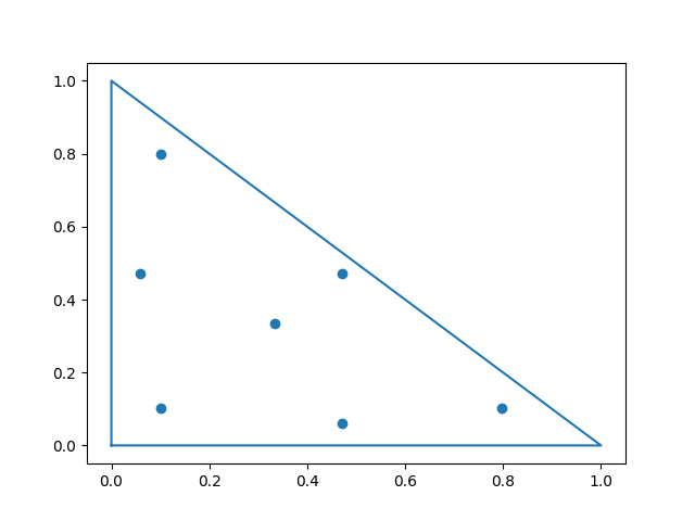
Example We discretize the problem with a continuous Galerkin ansatz space, and use a retriangulation with caps to approximate the truncation of the interaction set. We choose a seven-point quadrature rule with points Px and weights dx which is advantageous for the approximation of the truncated interaction set of a finite element, as the points lie close to the edges of the element [DElia2021].

import numpy as np
Px = np.array([[0.33333333333333, 0.33333333333333],
                [0.47014206410511, 0.47014206410511],
                [0.47014206410511, 0.05971587178977],
                [0.05971587178977, 0.47014206410511],
                [0.10128650732346, 0.10128650732346],
                [0.10128650732346, 0.79742698535309],
                [0.79742698535309, 0.10128650732346]])
dx = 0.5 * np.array([0.22500000000000,
                0.13239415278851,
                0.13239415278851,
                0.13239415278851,
                0.12593918054483,
                0.12593918054483,
                0.12593918054483])

The example configuration is set by the dictionary:

conf = {
     "ansatz": "CG",
     "approxBalls": {
         "method": "retriangulate"
     },
     "quadrature": {
         "outer": {
             "points": Px,
             "weights": dx
         },
         "inner": {
             "points": Px,
             "weights": dx
         },
         "touchingElements": {
              "method": "fractional",
              "ntensorGaussPoints": 4
         }
     },
     "verbose": True
 }

Note All options for the settings in kernel, function and conf can be printed by nlfem.show_options(). Empty dictionaries in the required form can be obtained from nlfem.get_empty_settings().

Assembly

Given the above settings the assembly of the nonlocal stiffness matrix is effected via

import nlfem
mesh, A = nlfem.stiffnessMatrix_fromArray(elements, elementLabels, vertices, kernel, conf)
f = nlfem.loadVector(mesh, forcing, conf)

The dictionary mesh contains information about the labeling of elements, vertices and dof. The labels of the degrees of freedom depend on the kernel (scalar or matrix-valued) and the ansatz space (continuous (CG) or discontinuous (DG) P1 elements). Therefore the function nlfem.stiffnessMatrix_fromArray() automatically deduces vertexLabels and dofLabels. A vertex is labeled according to the labels of the elements it belongs to and it is given the smallest of those element labels. The dof labels are identical to the vertexlabels for CG ansatz spaces and scalar-valued kernels. For DG ansatz spaces the labels are directly obtained from the element labels.

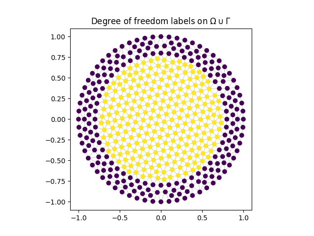
The labels of the degrees of freedom on the domain \(\Omega\) and the Dirchlet domain \(\Gamma^D\) are derived from the element labels and stored in mesh as dofLabels.

Omega = mesh["dofLabels"] > 0
Gamma = mesh["dofLabels"] < 0

Example In the given example we have a CG ansatz space and a scalar-valued kernel so that the dofLabels are identical to the vertexLabels.

plt.triplot(vertices[:, 0], vertices[:, 1], elements, color="black", linewidth=.2, alpha=.7)
plt.scatter(vertices[:, 0], vertices[:, 1], c=mesh["dofLabels"])
plt.title("DoF labels")
plt.gca().set_aspect('equal')
plt.savefig("doflabels.png")
plt.close()

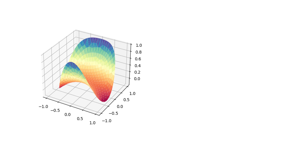
The solution of a Dirichlet-type problem requires the definition of Dirichlet data. The function below implements \(g(x) = x_1^2 x_2 + x_2^2\).

def g(vertices):
        return vertices[:, 0] ** 2 * vertices[:, 1] + vertices[:, 1] ** 2

Ultimately we can solve the nonlocal Dirichlet-type problem via

from scipy.sparse.linalg import cg
f_O = f[Omega]
A_OO = A[Omega][:, Omega]
A_OD = A[Omega][:, Gamma]
g_D = g(vertices[Gamma])
f_O -= A_OD.dot(g_D)

u = np.zeros(vertices.shape[0], dtype=float)
u[Omega] = cg(A_OO, f_O)[0]
u[Gamma] = g_D

fig = plt.figure(figsize=plt.figaspect(0.5))
ax = fig.add_subplot(1, 2, 1, projection='3d')
surf = ax.plot_trisurf(vertices[:, 0],vertices[:, 1], u, cmap=plt.cm.Spectral)
plt.savefig("solution.png")
plt.close()

Defining integral kernels

New kernels can be added to nlfem in the following way. Declare your kernel kernel_myKernel() in src/model.h and implement it in src/model.cpp. You kernel function has to exactly meet the interface of the function pointer model_kernel.

void (*model_kernel) (const double * x, long labelx,
const double * y,long labely,
const MeshType &mesh, double * kernel_val);

In order to be able to choose the kernel in the Python interface add an entry

{"myKernelName", kernel_myKernel}

to the map lookup_kernel in src/Cassemble.cpp.

[DElia2021]

D’Elia, M., Gunzburger, M., & Vollmann, C. (2021). A cookbook for approximating Euclidean balls and for quadrature rules in finite element methods for nonlocal problems. Mathematical Models and Methods in Applied Sciences, 31(08), 1505-1567.

[Klar2022]

Klar, M., Vollmann, C., & Schulz, V. (2022). nlfem: A flexible 2d Fem Code for Nonlocal Convection-Diffusion and Mechanics. arXiv preprint arXiv:2207.03921.

Python interface

nlfem.show_options()

Shows options for kernel, load and configuration settings. The kernel and forcing functions are imported directly from src/Cassemble.cpp.

nlfem.get_empty_settings()

Returns empty dictionaries which can be filled with values. Possible options can be printed via show_options().

nlfem.stiffnessMatrix_fromArray()

Computes the stiffness matrix corresponding to the nonlocal operator

\[-\mathcal{L}(\mathbf{u})(\mathbf{x}) = 2 \int_{B_{\delta}(\mathbf{x}) \cap \widehat{\Omega}}(\mathbf{C}_\delta(\mathbf{x}, \mathbf{y}) \mathbf{u}(\mathbf{x}) - \mathbf{C}_\delta(\mathbf{y}, \mathbf{x})\mathbf{u}(\mathbf{y})) d\mathbf{y},\]

on a given mesh. This function is a wrapper around stiffnessMatrix().

Parameters:

• elements – Numpy array containing the information about the elements. The values in the array "elements" are expected to be of datatype numpy.int.

• elementLabels – The values in the array "elementLabels" are expected to be of datatype numpy.int. Elements in the domain have positive labels. Elements in the nonlocal Dirichlet boundary have negative labels. For this purpose it does not matter which positive or negative number is used, and the kernels can depend on the element labels. The routine does not compute contributions of elements with label zero, i.e. they are ignored. The label zero can therefore be added to connect disconnected domains. The labels of the vertices are automatically derived from the element labels. In the case of Discontinuous Galerkin this means that the signs of the element labels and corresponding vertex labels coincide. In case of Continuous Galerkin this means that a vertex gets the smallest label of the non-zero labels of the adjacent elements.

• vertices – The values in the array "vertices" are supposed to be of type numpy.float64.

• kernel – The kernel is assumed to be a dictionary containing the keys "function", and "outputdim". The value of "function" is a string which contains the name of the kernel (e.g. “constant”). You find all available options in the function src/Cassemble.cpp/lookup_configuration(). The key "outputdim" describes the output dimension of the kernel function. In case of a scalar valued kernel this would be 1. In case of the kernel “linearPrototypeMicroelasticField” this would be 2 (find an example in examples/Test2D/testConfFull.py). Note, that the value of "outputdim" does not define the output dimension of the kernel, but describes it. The value has to be consistent with the definition of the corresponding kernel in src/model.cpp.

• configuration – Dictionary containing the configuration (find an example in examples/test2D/conf/testConfFull.py).

Return mesh:

Dictionary containing the mesh information. Can also be used for stiffnessMatrix() and loadVector().

Return A:

Matrix in scipy csr-sparse format of shape K x K where K = nVerts * outdim (Continuous Galerkin) or K = nElems * (dim+1) * outdim (Discontinuous Galerkin).

nlfem.stiffnessMatrix()

Computes the stiffness matrix corresponding to the nonlocal operator

\[-\mathcal{L}(\mathbf{u})(\mathbf{x}) = 2 \int_{B_{\delta}(\mathbf{x}) \cap \widehat{\Omega}}(\mathbf{C}_\delta(\mathbf{x}, \mathbf{y}) \mathbf{u}(\mathbf{x}) - \mathbf{C}_\delta(\mathbf{y}, \mathbf{x})\mathbf{u}(\mathbf{y})) d\mathbf{y},\]

on a given mesh. The input parameters are expected to be dictionaries. Find more information on the expected content in the examples/Test2D/conf/testConfFull.py. This function is a wrapper for the function par_assemble.

Parameters:

• mesh – Dictionary containing the mesh information (i.e. the keys "elements", "elementLabels", "vertices", and "vertexLabels"). The values in the arrays "elements", "elementLabels" and "vertexLabels" are expected to be of datatype numpy.int. The values in "vertices" are supposed to be of type numpy.float64. Elements in the domain have positive labels. Elements in the nonlocal Dirichlet boundary have negative labels. For this purpose it does not matter which positive or negative number is used, and the kernels can depend on the element labels. The labels of the elements should be consistent with the vertex labels. In the case of Discontinuous Galerkin this means that the signs of the element labels and corresponding vertex labels coincide. In case of Continuous Galerkin this means that elements with negative label have only vertices with negative label.

• kernel – The kernel is assumed to be a dictionary containing the keys "function", and "outputdim". The value of "function" is a string which contains the name of the kernel (e.g. “constant”). You find all available options in the function src/Cassemble.cpp/lookup_configuration(). The key "outputdim" describes the output dimension of the kernel function. In case of a scalar valued kernel this would be 1. In case of the kernel “linearPrototypeMicroelasticField” this would be 2 (find an example in examples/Test2D/testConfFull.py). Note, that the value of "outputdim" does not define the output dimension of the kernel, but describes it. The value has to be consistent with the definition of the corresponding kernel in src/model.cpp.

• configuration – Dictionary containing the configuration (find an example in examples/Test2D/conf/testConfFull.py).

Returns:

Matrix A in scipy csr-sparse format of shape K x K where K = nVerts * outdim (Continuous Galerkin) or K = nElems * (dim+1) * outdim (Discontinuous Galerkin).

nlfem.loadVector()

Computes load vector. The input parameters are expected to be dictionaries. Find more information on the expected content in the example/Test2D/testConfFull.py

Parameters:

• mesh – Dictionary containing the mesh information (i.e. the keys "elements", "elementLabels", "vertices", "vertexLabels" and "outdim"), where "outdim" is the output-dimension of the kernel. In this function the output dimension is read from "outdim", as no kernel is expected. The load cannot yet depend on label information.

• load – Dictionary containing the load information (find an example in testConfFull.py).

• configuration – Dictionary containing the configuration (find an example in examples/Test2D/conf/testConfFull.py).

Returns:

Vector f of shape K = nVerts * outdim (Continuous Galerkin) or K = nElems * (dim+1) * outdim (Discontinuous Galerkin)

Indices and tables

• Index

• Module Index

• Search Page